Internal caustics: Debye series v. ray tracing

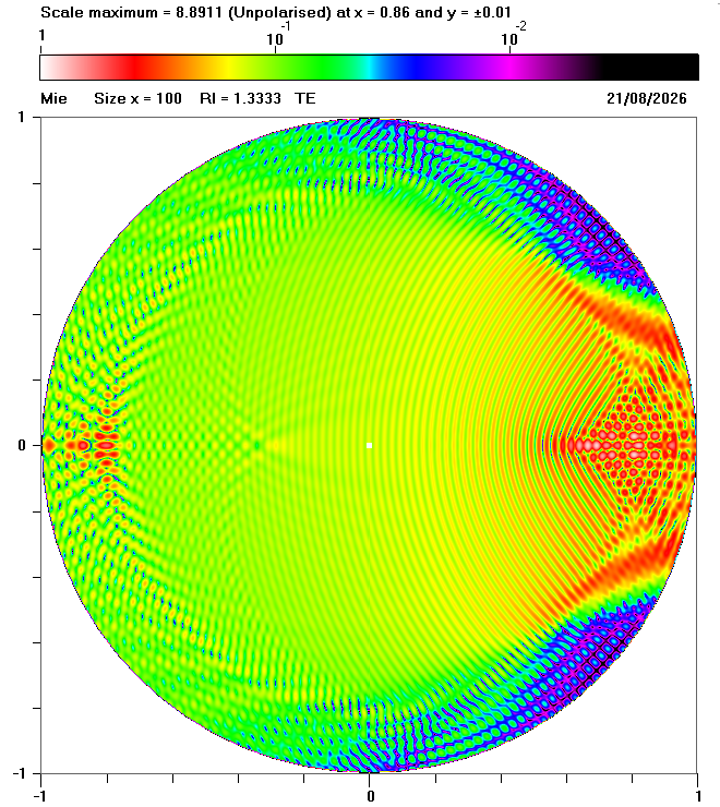
Fig. 1 Mie calculations showing the internal field for a sphere with size parameter x = 100, refractive index n = 1.3333 and TE polarization

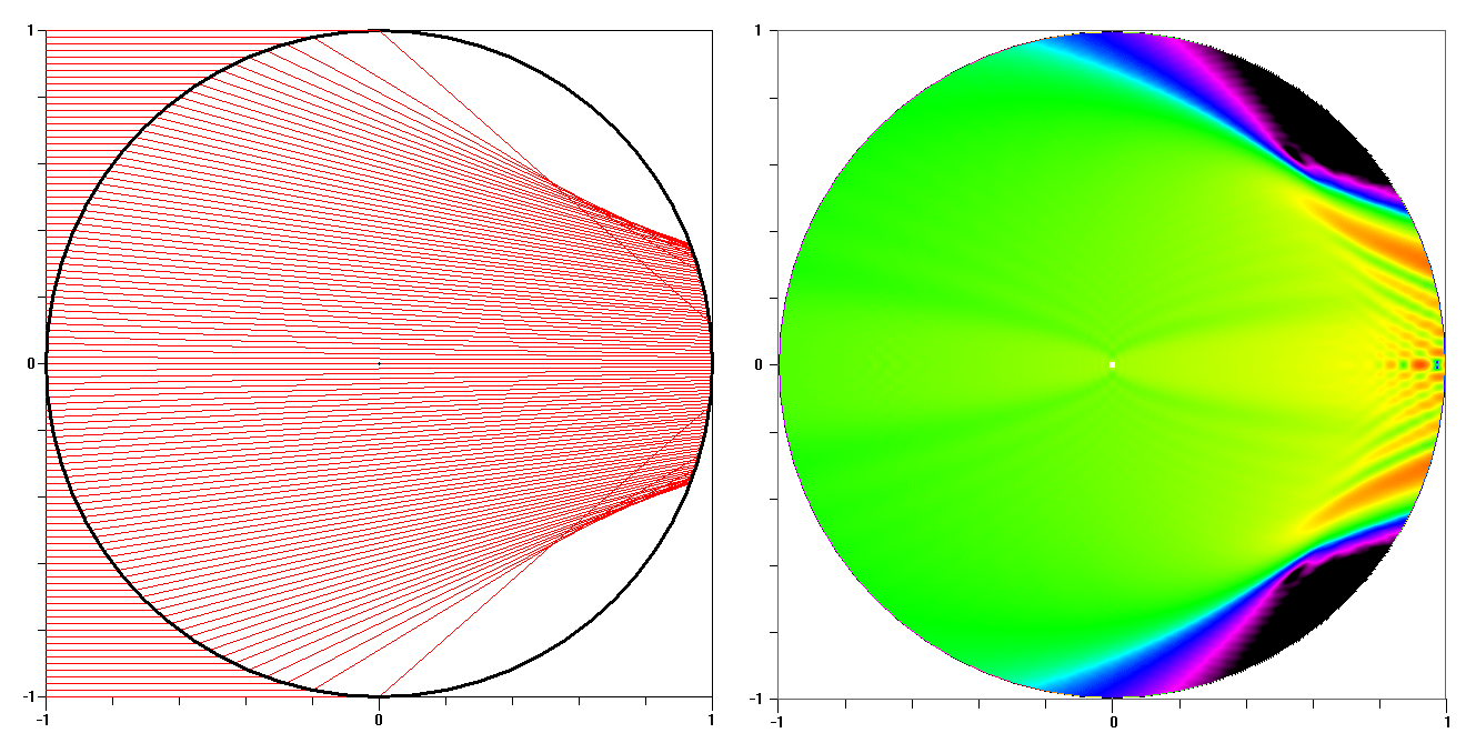
In order to explain the complicated patterns of internal fields, it can be helpful to compare the results of Mie calculations with the results of geometrical optics.   It is often even better to compare the results of Debye series calclulations with the results of ray tracing for a specified value of p where:

• p = 0 indicates light that is diffracted or reflected from the exterior of the sphere;
• p = 1 indicates light that is directly transmitted through the sphere;
• p = 2 indicates light that is subject to one internal reflection;
• p = 3 indicates light that is subject to two internal reflections;
• and so on ...

More generally, when p > 1, the light is subject to (p - 1) internal reflections.

By definition, calculations for p = 0 show no internal field because the incident light is either diffracted or reflected from the exterior of the sphere, indicating that no light enters the droplet.   On the other hand, the patterns of the internal field are very dependent on the value of p when p ≥ 1, as shown below.

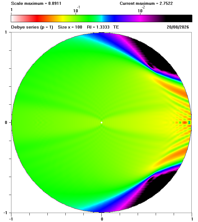
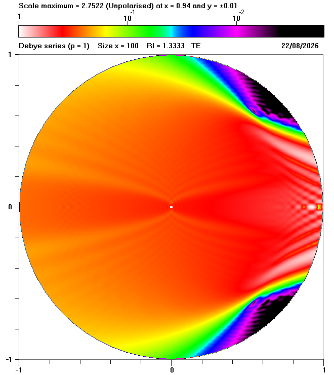
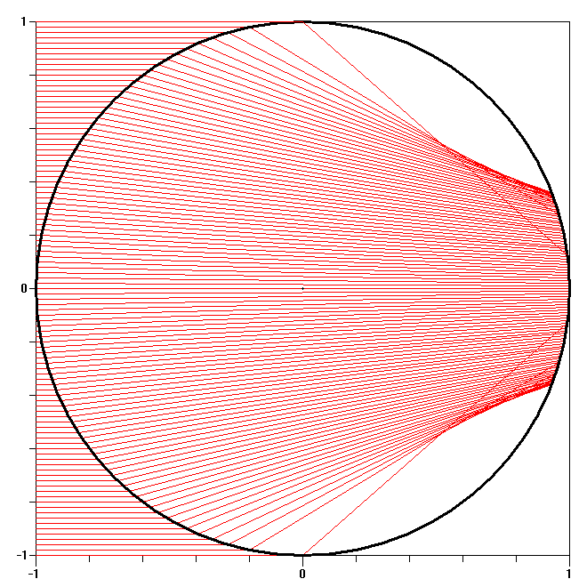
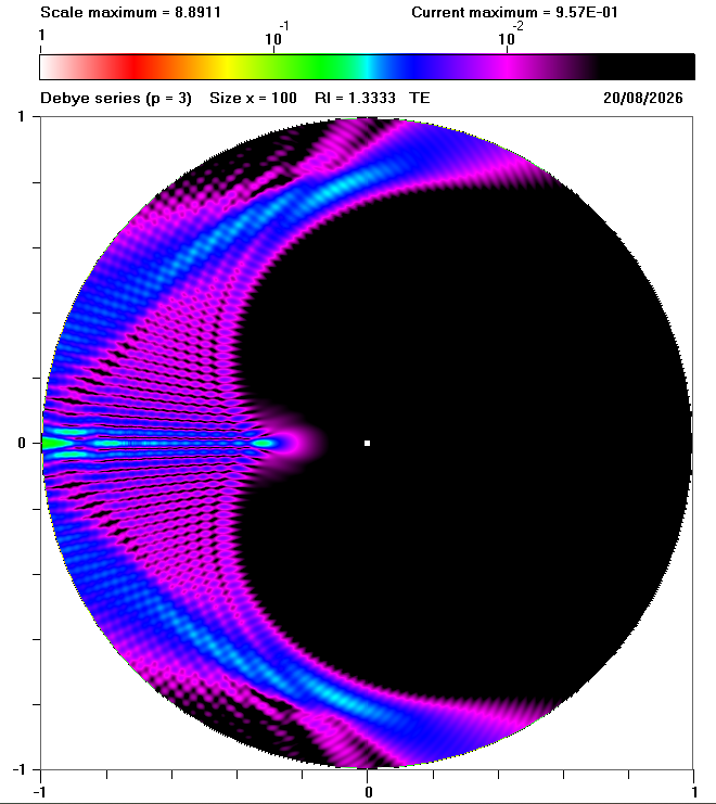
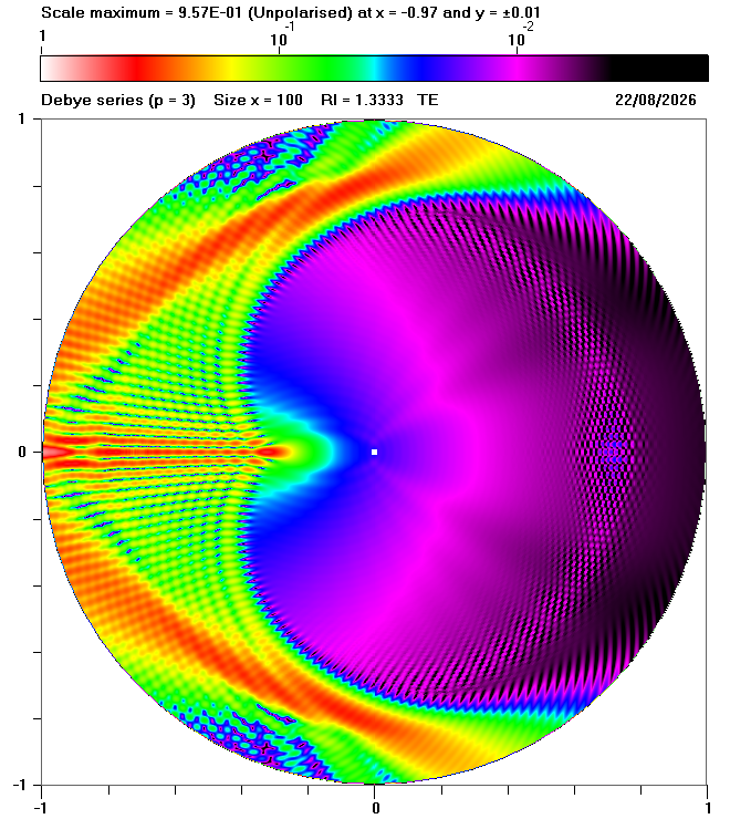
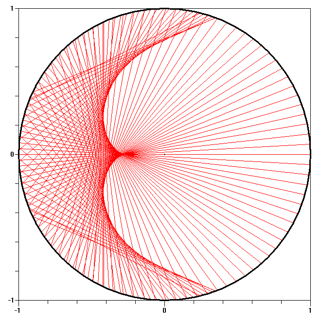
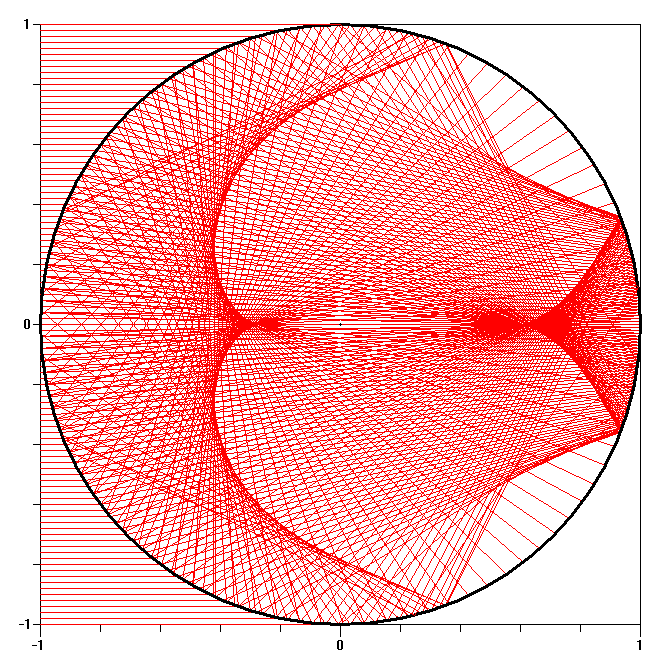
Each row of the following diagram show results for a sphere with size parameter x = 100, refractive index n = 1.3333 and TE polarization for a specific value of p, as defined below:

• The first column shows Debye results in which the intensity scale has been normalised to the peak value of 8.8911 corresponding to the Mie result shown in Fig. 1 above, thus maintaining the correct relationship with the other diagrams in the first column.
• The second column shows Debye results in which the intensity scale has been adjusted to the peak value of each individual diagrams (e.g. 2.7522 for p = 1 and 5.8939 for p = 2 ), thus emphasising weaker features in each diagram.
• The third column shows ray tracing for the specified value of p.
• The fourth column shows ray tracing for the cumulative values from p = 1 to the specified value of p.

Debye (normalised)	Debye	Ray tracing for specified value of p	Ray tracing for p = 1 to specified value of p
p = 1	p = 1	p = 1	p = 1
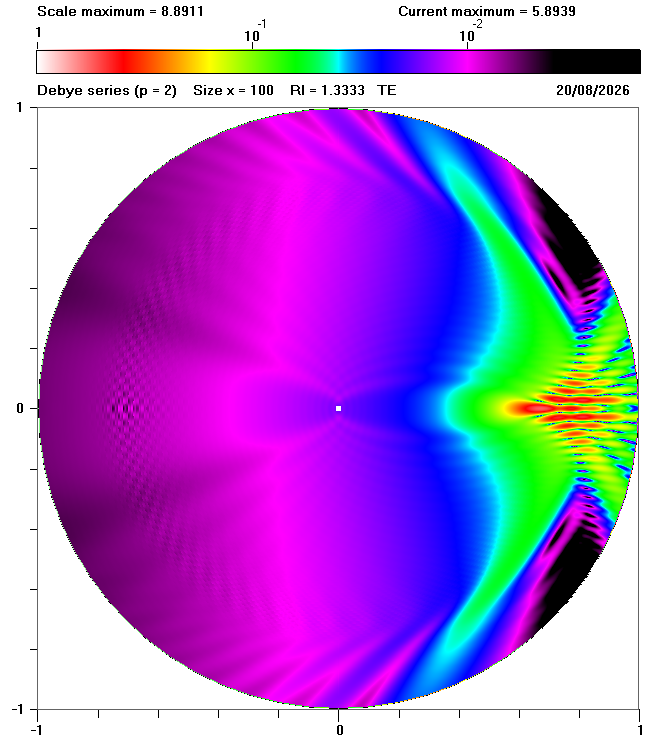p = 2	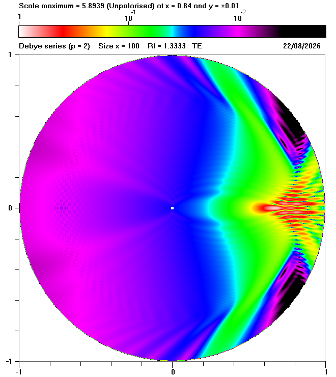p = 2	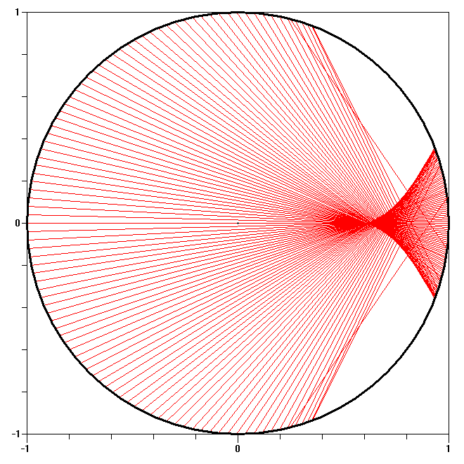p = 2	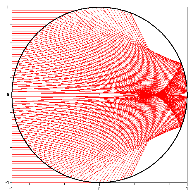p = 1 to p = 2
p = 3	p = 3	p = 3	p = 1 to p = 3
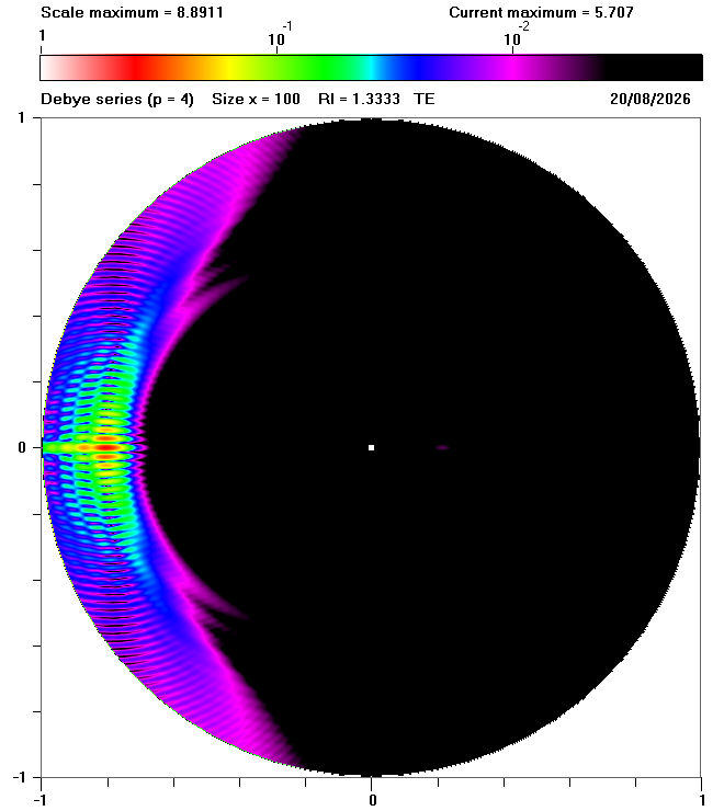p = 4	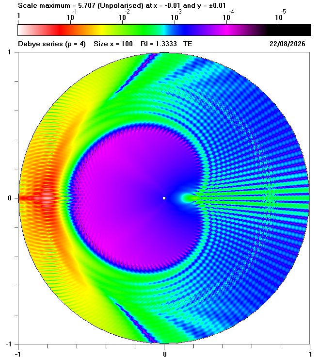p = 4	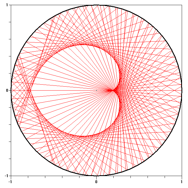p = 4	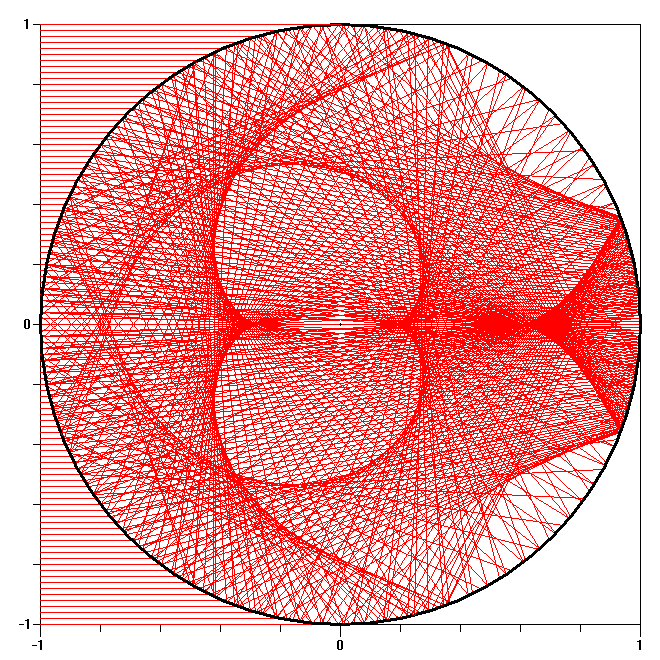p = 1 to p = 4
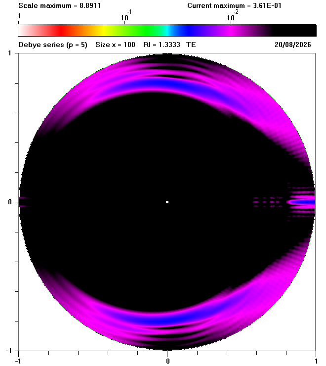p = 5	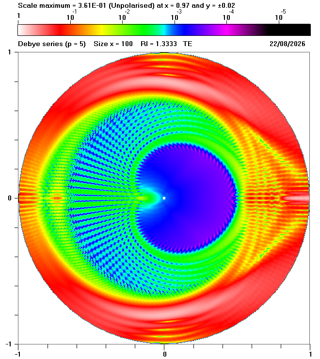p = 5	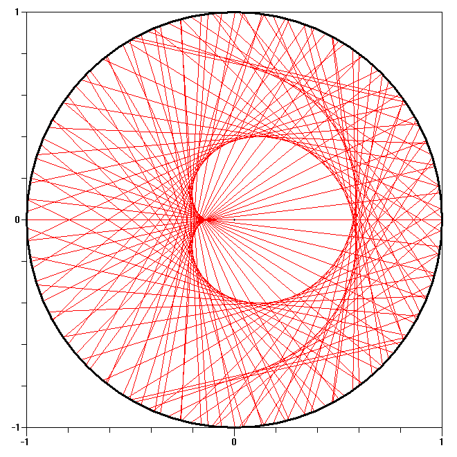p = 5	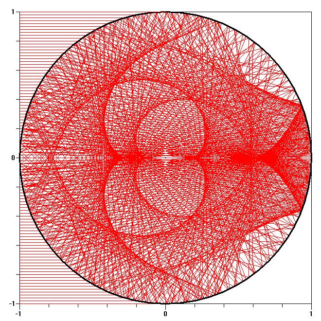p = 1 to p = 5
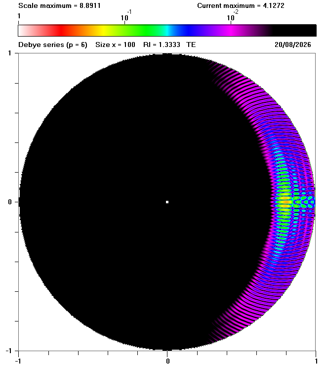p = 6	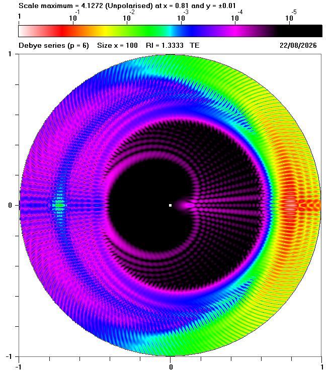p = 6	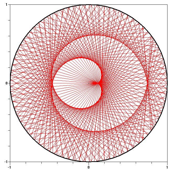p = 6	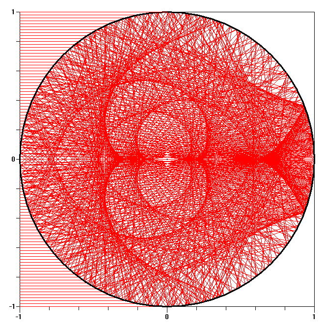p = 1 to p = 6
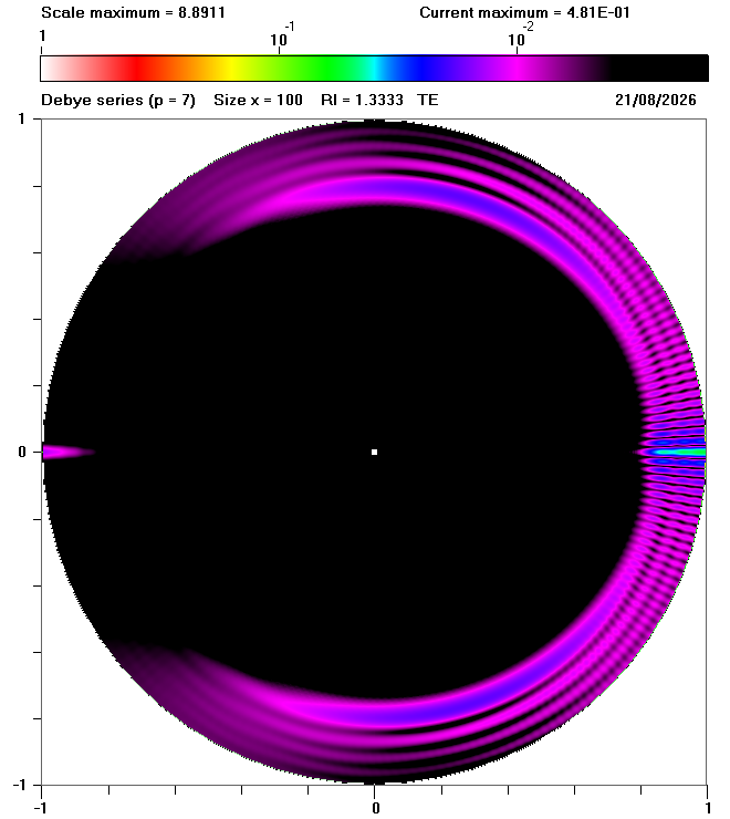p = 7	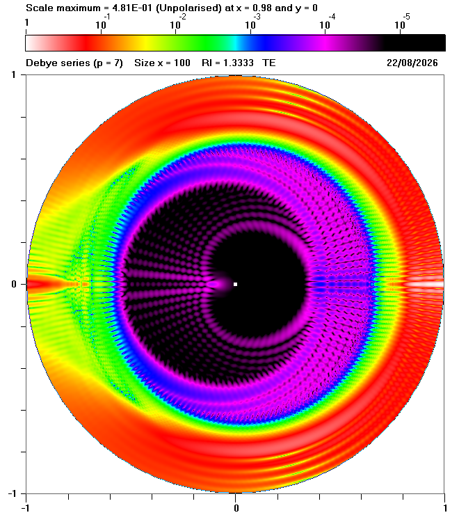p = 7	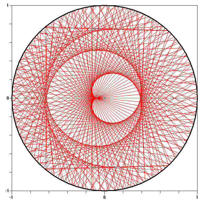p = 7	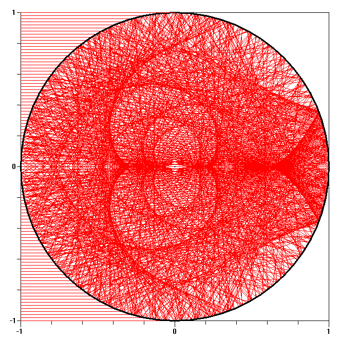p = 1 to p = 7
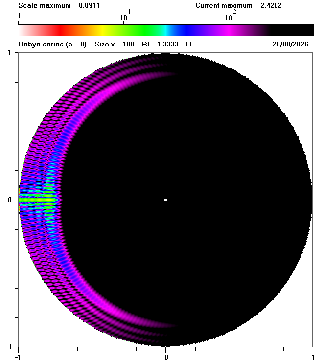p = 8	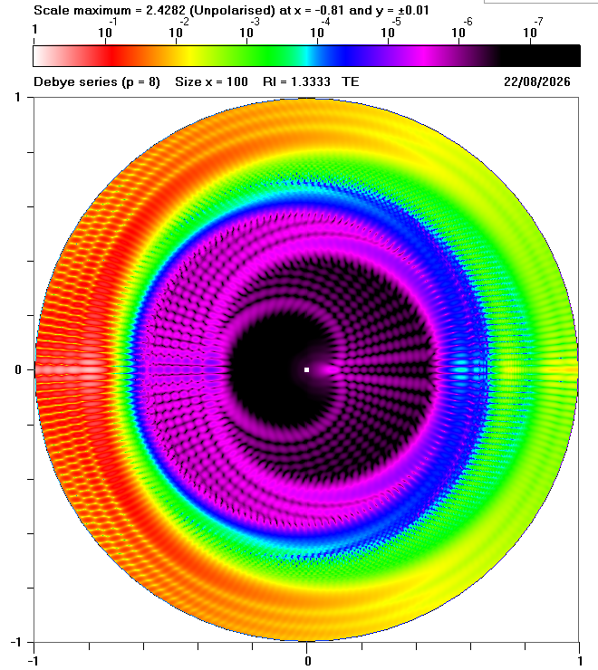p = 8	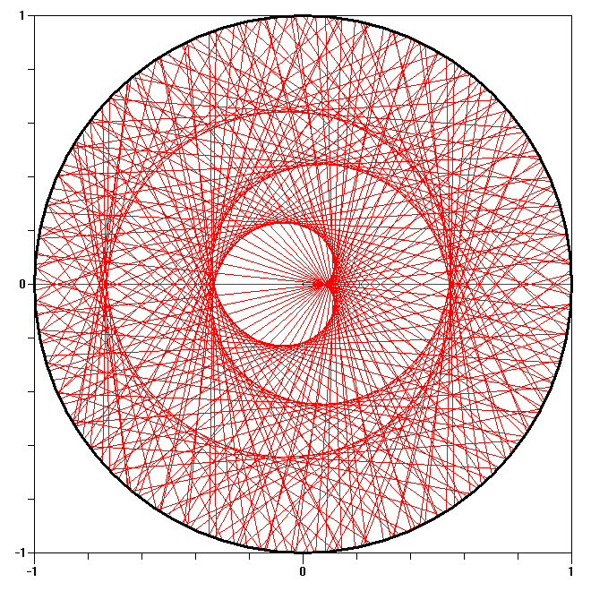p = 8	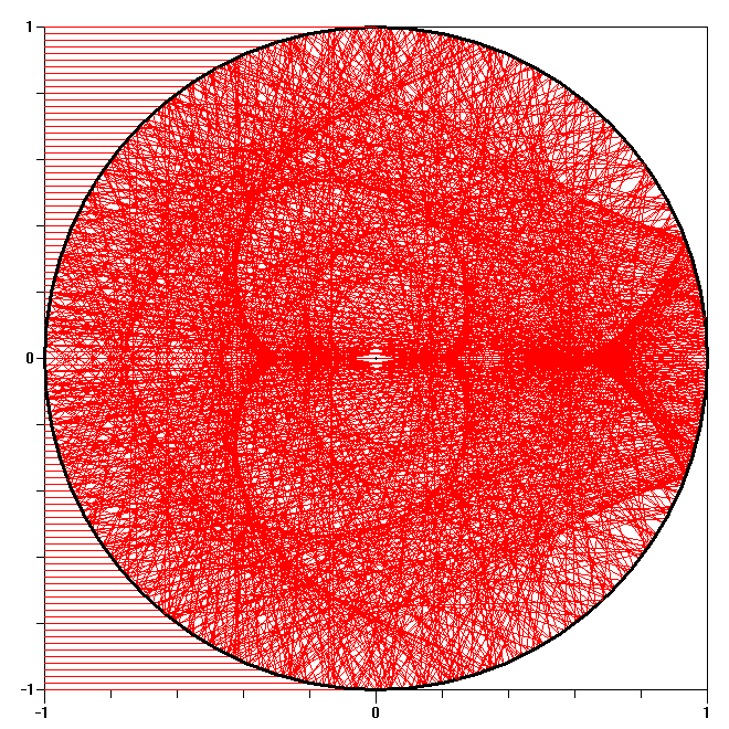p = 1 to p = 8

Fig. 2   Comparisons of Debye calculations and ray tracing for specific values of p

Caustics mark the boundaries between areas where multiple rays contribute to the internal field and areas where no (or very few) geometrical rays can reach.   It is easy to identify caustics in the ray tracing diagrams: for example, caustics occur at the top right and bottom right of the diagrams for p = 1.   Fig. 2 also shows that, for p > 1, ray tracing generates caustics with very complicated shapes.   It is interesting to see that these complicated shapes are replicated in the Debye calculations - especially in the second column of Fig. 2.   Although the caustics are very obvious in the ray tracing diagrams, many of these caustics result in enhancements that are so weak that they are not visible in the first column of Fig. 2.

However, it would be wrong to assume that areas where there are no geometrical rays correspond to zero intensity.   Similarly, caustics formed by a multiplicity of rays do not necessarily correspond to maximum intensity.   As shown by the animation in Fig. 3 below, the internal fields for p = 1 extend well beyond the boundaries defined by the caustics and the maximum intensity does not coincide exactly with the caustics.   This is analogous to the rainbow where ray tracing predicts infinite intensity at the caustic together with an immediate transition to zero intensity, whereas Debye calculations exhibit a a rainbow maximum at a slightly different scattering angle, with a gradual reduction in intensity in the "shadow zone".

Fig. 3   Animation comparing the diagrams for p = 1 in the second and third columns of Fig. 2.